Radon Example

Author

Brandon T. Willard

Date

2019-09-08

Introduction

In this example we’ll create a model “optimizer” that approximates the re-centering and re-scaling commonly demonstrated on a hierarchical normal model for the radon dataset. This optimization is symbolic and effectively produces another equivalent model with better sampling properties.

A similar example already exists in Theano and PyMC3; this example will operate on TensorFlow (TF) graphs via PyMC4 and approximate the same optimization using a very different approach targeted toward the log-likelihood graph.

To get started, we need to download the radon dataset. We do this setup in python-setup and radon-data-download, then we define the initial model in pymc4-radon-model.

import numpy as np
import pandas as pd
import tensorflow as tf

import pymc4 as pm
import arviz as az

data = pd.read_csv('https://github.com/pymc-devs/pymc3/raw/master/pymc3/examples/data/radon.csv')

county_names = data.county.unique()
county_idx = data['county_code'].values.astype(np.int32)

@pm.model
def hierarchical_model(data, county_idx):
    # Hyperpriors
    mu_a = yield pm.Normal('mu_alpha', mu=0., sigma=1)
    sigma_a = yield pm.HalfCauchy('sigma_alpha', beta=1)
    mu_b = yield pm.Normal('mu_beta', mu=0., sigma=1)
    sigma_b = yield pm.HalfCauchy('sigma_beta', beta=1)

    # Intercept for each county, distributed around group mean mu_a
    a = yield pm.Normal('alpha', mu=mu_a, sigma=sigma_a, plate=len(data.county.unique()))
    # Intercept for each county, distributed around group mean mu_a
    b = yield pm.Normal('beta', mu=mu_b, sigma=sigma_b, plate=len(data.county.unique()))

    # Model error
    eps = yield pm.HalfCauchy('eps', beta=1)

    # Expected value
    #radon_est = a[county_idx] + b[county_idx] * data.floor.values
    radon_est = tf.gather(a, county_idx) + tf.gather(
        b, county_idx) * data.floor.values

    # Data likelihood
    y_like = yield pm.Normal('y_like', mu=radon_est, sigma=eps, observed=data.log_radon)


init_num_chains = 50
model = hierarchical_model(data, county_idx)

In pymc4-radon-model-sample, we estimate the model using the sample routine from PyMC4’s Radon example Notebook (reproduced in pymc4-sample-function). The same plots from the aforementioned notebook are also reproduced here in fig:pymc4-radon-plot-energy and fig:pymc4-radon-plot-trace.

def sample(model, init_num_chains=50, num_samples=500, burn_in=500):
    init_num_chains = 50
    pm4_trace, _ = pm.inference.sampling.sample(
        model, num_chains=init_num_chains, num_samples=10, burn_in=10, step_size=1., xla=True)
    for i in range(3):
        step_size_ = []
        for _, x in pm4_trace.items():
            std = tf.math.reduce_std(x, axis=[0, 1])
            step_size_.append(
                std[tf.newaxis, ...] * tf.ones([init_num_chains] + std.shape, dtype=std.dtype))
        pm4_trace, _ = pm.inference.sampling.sample(
            model, num_chains=init_num_chains, num_samples=10 + 10*i, burn_in=10 + 10*i,
            step_size=step_size_, xla=True)

    num_chains = 5
    step_size_ = []
    for _, x in pm4_trace.items():
        std = tf.math.reduce_std(x, axis=[0, 1])
        step_size_.append(
            std[tf.newaxis, ...] * tf.ones([num_chains]+std.shape, dtype=std.dtype))

    pm4_trace, sample_stat = pm.inference.sampling.sample(
        model, num_chains=num_chains, num_samples=num_samples, burn_in=burn_in,
        step_size=step_size_, xla=True)

    az_trace = pm.inference.utils.trace_to_arviz(pm4_trace, sample_stat)

    return az_trace

az_trace = sample(model)

import matplotlib.pyplot as plt

import seaborn as sns

from matplotlib import rcParams


rcParams['figure.figsize'] = (11.7, 8.27)

# plt.rc('text', usetex=True)
sns.set_style("whitegrid")
sns.set_context("paper")

_ = az.plot_energy(az_trace)

Fig. 3 Pre-transform MCMC energy

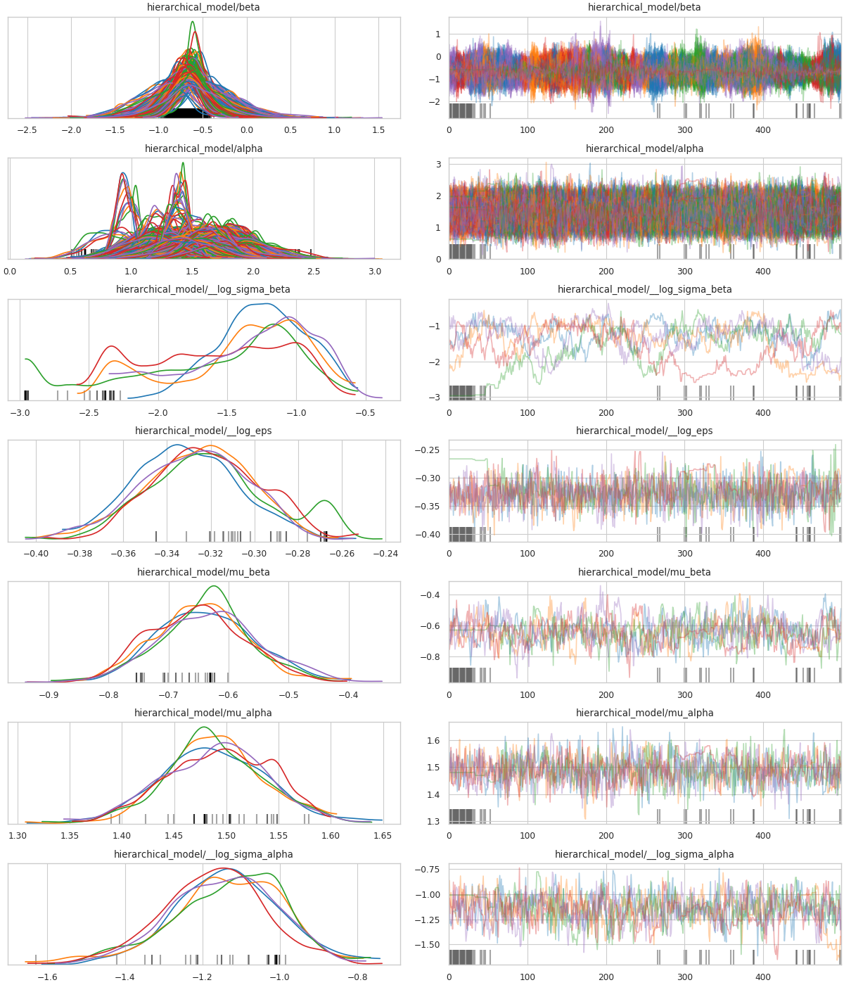
Fig. 4 Pre-transform MCMC trace

The Model’s Log-likelihood Graph

In order to apply our optimization, we need to obtain a graph of the log-likelihood function generated by the model in pymc4-radon-model. With the graph in-hand, we can perform the re-centering and re-scaling transform–in log-space–and produce a new log-likelihood graph that improves sampling.

This exercise introduces the TensorFlow function-graph backed by the class tensorflow.python.framework.func_graph.FuncGraph. FuncGraph is a subclass of the regular Graph objects upon which symbolic-pymc indirectly operates. Just like Theano’s FunctionGraphs, FuncGraphsimply specializes a generic graph by specifying which constituent tensors are considered inputs and outputs.

In logp-func, we use PyMC4’s internal mechanisms to build the log-likelihood function for our model and a corresponding list of initial values for the parameters.

state = None
observed = None

logpfn, init = pm.inference.sampling.build_logp_function(model,
                                                         state=state,
                                                         observed=observed)

From here we need FuncGraphs for each input to logpfn. Since logpfn is a tensorflow.python.eager.def_function.Functioninstance, every time it’s called with a specific tensor it may create a new function-object with its own FuncGraph. In other words, it dynamically generates function objects based on the inputs it’s given.

This specialization process can be performed manually using logpfn.get_concrete_function(*args), which necessarily produces a tensorflow.python.eager.function.ConcreteFunctionwith the desired FuncGraph. fgraph-specializations creates and extracts these two objects.

logpfn_cf = logpfn.get_concrete_function(*init.values())
logpfn_fg = logpfn_cf.graph

The outputs are now available in graph form as logpfn_fg.outputs.

The Log-space Transform

Consider the following two equivalent hierarchical models,

\[\begin{split}\begin{equation} \begin{gathered} Y = X + \epsilon, \quad \epsilon \sim \operatorname{N}\left(0, \sigma^2\right) \\ X \sim \operatorname{N}\left(\mu, \tau^2\right) \end{gathered} \label{eq:model-1} \end{equation}\end{split}\]

\[\begin{split}\begin{equation} \begin{gathered} Y = \mu + \tau \cdot \tilde{X} + \epsilon, \quad \epsilon \sim \operatorname{N}\left(0, \sigma^2\right) \\ \tilde{X} \sim \operatorname{N}\left(0, 1\right) \;. \end{gathered} \label{eq:model-2} \end{equation}\end{split}\]

Models eq:model-1 and eq:model-2 are represented in (log) measure space, respectively, as follows:

\[\begin{split}\begin{align} \log p(Y, X) &= \log P(Y\mid X) + \log P(X) \nonumber \\ &= C - \frac{1}{2} \left(\frac{y}{\sigma} - \frac{x}{\sigma}\right)^2 - \frac{1}{2} \left(\frac{x}{\tau} - \frac{\mu}{\tau}\right)^2 \label{eq:log-model-1} \\ &= \tilde{C} - \frac{1}{2} \left(\frac{y}{\sigma} - \frac{\mu - \tau \cdot \tilde{x}}{\sigma}\right)^2 - \frac{1}{2} \tilde{x}^2 \label{eq:log-model-2} \;. \end{align}\end{split}\]

Via term rewriting, Equation eq:log-model-2 is produced–in part–by applying the replacement rule \(x \to \mu + \tau \cdot \tilde{x}\) to Equation eq:log-model-1, i.e.

\[\begin{align*} \tilde{C} - \frac{1}{2} \left(\frac{y}{\sigma} - \frac{\mu + \tau \cdot \tilde{x}}{\sigma}\right)^2 - \frac{1}{2} \left(\frac{\mu + \tau \cdot \tilde{x}}{\tau} - \frac{\mu}{\tau}\right)^2 \;. \end{align*}\]

For consistency, the transform must also be applied to the \(dx\) term where/when-ever it is considered.

After a few algebraic simplifications, one obtains the exact form of Equation eq:log-model-2.

Creating the miniKanren Goals

symbolic-pymc is designed to use miniKanren as a means of specifying mathematical relations. The degree to which an implementation of a mathematical relation upholds its known characteristics is–of course–always up to the developer. For the needs of PPLs like PyMC4, we can’t reasonably expect–or provide–capabilities at the level of automatic theorem proving or every relevant state-of-the-art symbolic math routine.

Even so, we do expect that some capabilities from within those more advanced areas of symbolic computing will eventually be required–or necessary–and we want to build on a foundation that allows them to be integrated and/or simply expressed. We believe that miniKanren is a great foundation for such work due to the core concepts it shares with symbolic computation, as well as its immense flexibility. It also maintains an elegant simplicity and is amenable to developer intervention at nearly all levels–often without the need for low- or DSL-level rewrites.

User-level development in miniKanren occurs within its DSL, which is a succinct relational/logic programming paradigm that–in our case–is entirely written in Python. This DSL provides primitive goals that can be composed and eventually evaluated by the run function. We refer the reader to any one of the many great introductions to miniKanren available at http://minikanren.org, or, for the specific Python package used here: this simple introduction.

For the matter at hand, we need to create goals that implement the substitution described above. The first step is to understand the exact TF graphs involved, and the best way to do that is to construct the relevant graph objects, observe them directly, and build “patterns” that match their general forms. Patterns are built with symbolic-pymc meta objects obtained from the mt helper “namespace”. Wherever we want to leave room for variation/ambiguity, we use a “logic variable” instead of an explicit TF (meta) object. Logic variables are created with var() and can optionally be given a string “name” argument that identifies them globally as a singleton-like object.

Inspecting the TF Graphs

In our case, the log-density returned by PyMC4–via the TensorFlow Probability library (TFP)– uses tf.math.squared_difference to construct the “squared error” term in the exponential of a normal distribution. This term contains everything we need to construct the substitution as a pair of TF graph objects.

tfp-normal-log-lik-graph shows the graph produced by a normal distribution in TFP.

import tensorflow_probability as tfp

from tensorflow.python.eager.context import graph_mode
from tensorflow.python.framework.ops import disable_tensor_equality

from symbolic_pymc.tensorflow.printing import tf_dprint


disable_tensor_equality()

with graph_mode(), tf.Graph().as_default() as test_graph:
    mu_tf = tf.compat.v1.placeholder(tf.float32, name='mu',
                                     shape=tf.TensorShape([None]))
    tau_tf = tf.compat.v1.placeholder(tf.float32, name='tau',
                                      shape=tf.TensorShape([None]))

    normal_tfp = tfp.distributions.normal.Normal(mu_tf, tau_tf)

    value_tf = tf.compat.v1.placeholder(tf.float32, name='value',
                                        shape=tf.TensorShape([None]))

    normal_log_lik = normal_tfp.log_prob(value_tf)

tf_dprint(normal_log_lik)

Tensor(Sub):0,      dtype=float32,  shape=[None],   "Normal_1/log_prob/sub:0"
|  Tensor(Mul):0,   dtype=float32,  shape=[None],   "Normal_1/log_prob/mul:0"
|  |  Tensor(Const):0,      dtype=float32,  shape=[],       "Normal_1/log_prob/mul/x:0"
|  |  |  -0.5
|  |  Tensor(SquaredDifference):0,  dtype=float32,  shape=[None],   "Normal_1/log_prob/SquaredDifference:0"
|  |  |  Tensor(RealDiv):0, dtype=float32,  shape=[None],   "Normal_1/log_prob/truediv:0"
|  |  |  |  Tensor(Placeholder):0,  dtype=float32,  shape=[None],   "value:0"
|  |  |  |  Tensor(Placeholder):0,  dtype=float32,  shape=[None],   "tau:0"
|  |  |  Tensor(RealDiv):0, dtype=float32,  shape=[None],   "Normal_1/log_prob/truediv_1:0"
|  |  |  |  Tensor(Placeholder):0,  dtype=float32,  shape=[None],   "mu:0"
|  |  |  |  Tensor(Placeholder):0,  dtype=float32,  shape=[None],   "tau:0"
|  Tensor(AddV2):0, dtype=float32,  shape=[None],   "Normal_1/log_prob/add:0"
|  |  Tensor(Const):0,      dtype=float32,  shape=[],       "Normal_1/log_prob/add/x:0"
|  |  |  0.9189385
|  |  Tensor(Log):0,        dtype=float32,  shape=[None],   "Normal_1/log_prob/Log:0"
|  |  |  Tensor(Placeholder):0,     dtype=float32,  shape=[None],   "tau:0"

Instead of looking for the entire log-likelihood graph for a distribution, we can focus on only the SquaredDifference operators, since they contain all the relevant terms for our transformation.

More specifically, if we can identify “chains” of such terms, i.e. SquaredDifference(y, x)and SquaredDifference(x, mu), then we might be able to assume that the corresponding subgraph was formed from such a hierarchical normal model.

show-squared-diff-terms shows the SquaredDifferencesub-graphs in the log-likelihood graph for our radon model. It demonstrates two instances of said SquaredDifference”chains”: they involve tensors named values_5 and values_1.

square_diff_outs = [o.outputs[0] for o in logpfn_fg.get_operations()
                    if o.type == 'SquaredDifference' or o.type.startswith('Gather')]

for t in square_diff_outs:
    tf_dprint(t)

Tensor(GatherV2):0, dtype=float32,  shape=[919],    "GatherV2:0"
|  Tensor(Placeholder):0,   dtype=float32,  shape=[85],     "values_1:0"
|  Tensor(Const):0, dtype=int32,    shape=[919],    "GatherV2/indices:0"
|  |  [ 0  0  0 ... 83 84 84]
|  Tensor(Const):0, dtype=int32,    shape=[],       "GatherV2/axis:0"
|  |  0
Tensor(GatherV2):0, dtype=float32,  shape=[919],    "GatherV2_1:0"
|  Tensor(Placeholder):0,   dtype=float32,  shape=[85],     "values_3:0"
|  Tensor(Const):0, dtype=int32,    shape=[919],    "GatherV2_1/indices:0"
|  |  [ 0  0  0 ... 83 84 84]
|  Tensor(Const):0, dtype=int32,    shape=[],       "GatherV2_1/axis:0"
|  |  0
Tensor(SquaredDifference):0,        dtype=float32,  shape=[],       "Normal_5/log_prob/SquaredDifference:0"
|  Tensor(RealDiv):0,       dtype=float32,  shape=[],       "Normal_5/log_prob/truediv:0"
|  |  Tensor(Placeholder):0,        dtype=float32,  shape=[],       "values_0:0"
|  |  Tensor(Const):0,      dtype=float32,  shape=[],       "Normal/scale:0"
|  |  |  1.
|  Tensor(RealDiv):0,       dtype=float32,  shape=[],       "Normal_5/log_prob/truediv_1:0"
|  |  Tensor(Const):0,      dtype=float32,  shape=[],       "Normal/loc:0"
|  |  |  0.
|  |  Tensor(Const):0,      dtype=float32,  shape=[],       "Normal/scale:0"
|  |  |  1.
Tensor(SquaredDifference):0,        dtype=float32,  shape=[],       "Normal_1_1/log_prob/SquaredDifference:0"
|  Tensor(RealDiv):0,       dtype=float32,  shape=[],       "Normal_1_1/log_prob/truediv:0"
|  |  Tensor(Placeholder):0,        dtype=float32,  shape=[],       "values_6:0"
|  |  Tensor(Const):0,      dtype=float32,  shape=[],       "Normal_1/scale:0"
|  |  |  1.
|  Tensor(RealDiv):0,       dtype=float32,  shape=[],       "Normal_1_1/log_prob/truediv_1:0"
|  |  Tensor(Const):0,      dtype=float32,  shape=[],       "Normal_1/loc:0"
|  |  |  0.
|  |  Tensor(Const):0,      dtype=float32,  shape=[],       "Normal_1/scale:0"
|  |  |  1.
Tensor(SquaredDifference):0,        dtype=float32,  shape=[85],     "SampleNormal_2_1/log_prob/Normal_2/log_prob/SquaredDifference:0"
|  Tensor(RealDiv):0,       dtype=float32,  shape=[85],     "SampleNormal_2_1/log_prob/Normal_2/log_prob/truediv:0"
|  |  Tensor(Transpose):0,  dtype=float32,  shape=[85],     "SampleNormal_2_1/log_prob/transpose:0"
|  |  |  Tensor(Reshape):0, dtype=float32,  shape=[85],     "SampleNormal_2_1/log_prob/Reshape:0"
|  |  |  |  Tensor(Placeholder):0,  dtype=float32,  shape=[85],     "values_1:0"
|  |  |  |  Tensor(Const):0,        dtype=int32,    shape=[1],      "SampleNormal_2_1/log_prob/Reshape/shape:0"
|  |  |  |  |  [85]
|  |  |  Tensor(Const):0,   dtype=int32,    shape=[1],      "SampleNormal_2_1/log_prob/transpose/perm:0"
|  |  |  |  [0]
|  |  Tensor(Exp):0,        dtype=float32,  shape=[],       "exp_1/forward/Exp:0"
|  |  |  Tensor(Placeholder):0,     dtype=float32,  shape=[],       "values_5:0"
|  Tensor(RealDiv):0,       dtype=float32,  shape=[],       "SampleNormal_2_1/log_prob/Normal_2/log_prob/truediv_1:0"
|  |  Tensor(Placeholder):0,        dtype=float32,  shape=[],       "values_0:0"
|  |  Tensor(Exp):0,        dtype=float32,  shape=[],       "exp_1/forward/Exp:0"
|  |  |  ...
Tensor(SquaredDifference):0,        dtype=float32,  shape=[85],     "SampleNormal_3_1/log_prob/Normal_3/log_prob/SquaredDifference:0"
|  Tensor(RealDiv):0,       dtype=float32,  shape=[85],     "SampleNormal_3_1/log_prob/Normal_3/log_prob/truediv:0"
|  |  Tensor(Transpose):0,  dtype=float32,  shape=[85],     "SampleNormal_3_1/log_prob/transpose:0"
|  |  |  Tensor(Reshape):0, dtype=float32,  shape=[85],     "SampleNormal_3_1/log_prob/Reshape:0"
|  |  |  |  Tensor(Placeholder):0,  dtype=float32,  shape=[85],     "values_3:0"
|  |  |  |  Tensor(Const):0,        dtype=int32,    shape=[1],      "SampleNormal_3_1/log_prob/Reshape/shape:0"
|  |  |  |  |  [85]
|  |  |  Tensor(Const):0,   dtype=int32,    shape=[1],      "SampleNormal_3_1/log_prob/transpose/perm:0"
|  |  |  |  [0]
|  |  Tensor(Exp):0,        dtype=float32,  shape=[],       "exp_2_1/forward/Exp:0"
|  |  |  Tensor(Placeholder):0,     dtype=float32,  shape=[],       "values_2:0"
|  Tensor(RealDiv):0,       dtype=float32,  shape=[],       "SampleNormal_3_1/log_prob/Normal_3/log_prob/truediv_1:0"
|  |  Tensor(Placeholder):0,        dtype=float32,  shape=[],       "values_6:0"
|  |  Tensor(Exp):0,        dtype=float32,  shape=[],       "exp_2_1/forward/Exp:0"
|  |  |  ...
Tensor(SquaredDifference):0,        dtype=float32,  shape=[919],    "Normal_4_1/log_prob/SquaredDifference:0"
|  Tensor(RealDiv):0,       dtype=float32,  shape=[919],    "Normal_4_1/log_prob/truediv:0"
|  |  Tensor(Const):0,      dtype=float32,  shape=[919],    "Normal_4_1/log_prob/value:0"
|  |  |  [0.8329091 0.8329091 1.0986123 ... 1.6292405 1.3350011 1.0986123]
|  |  Tensor(Exp):0,        dtype=float32,  shape=[],       "exp_3_1/forward/Exp:0"
|  |  |  Tensor(Placeholder):0,     dtype=float32,  shape=[],       "values_4:0"
|  Tensor(RealDiv):0,       dtype=float32,  shape=[919],    "Normal_4_1/log_prob/truediv_1:0"
|  |  Tensor(AddV2):0,      dtype=float32,  shape=[919],    "add:0"
|  |  |  Tensor(GatherV2):0,        dtype=float32,  shape=[919],    "GatherV2:0"
|  |  |  |  Tensor(Placeholder):0,  dtype=float32,  shape=[85],     "values_1:0"
|  |  |  |  Tensor(Const):0,        dtype=int32,    shape=[919],    "GatherV2/indices:0"
|  |  |  |  |  [ 0  0  0 ... 83 84 84]
|  |  |  |  Tensor(Const):0,        dtype=int32,    shape=[],       "GatherV2/axis:0"
|  |  |  |  |  0
|  |  |  Tensor(Mul):0,     dtype=float32,  shape=[919],    "mul:0"
|  |  |  |  Tensor(GatherV2):0,     dtype=float32,  shape=[919],    "GatherV2_1:0"
|  |  |  |  |  Tensor(Placeholder):0,       dtype=float32,  shape=[85],     "values_3:0"
|  |  |  |  |  Tensor(Const):0,     dtype=int32,    shape=[919],    "GatherV2_1/indices:0"
|  |  |  |  |  |  [ 0  0  0 ... 83 84 84]
|  |  |  |  |  Tensor(Const):0,     dtype=int32,    shape=[],       "GatherV2_1/axis:0"
|  |  |  |  |  |  0
|  |  |  |  Tensor(Const):0,        dtype=float32,  shape=[919],    "mul/y:0"
|  |  |  |  |  [1. 0. 0. ... 0. 0. 0.]
|  |  Tensor(Exp):0,        dtype=float32,  shape=[],       "exp_3_1/forward/Exp:0"
|  |  |  ...

The names in the TFP graph are not based on the PyMC4 model objects, so, to make the graph output slightly more interpretable, model-names-to-tfp-names attempts to re-associate the TF and PyMC4 object names.

from pprint import pprint

tfp_names_to_pymc = {i.name: k for i, k in zip(logpfn_cf.structured_input_signature[0], init.keys())}
pymc_names_to_tfp = {v: k for k, v in tfp_names_to_pymc.items()}

alpha_tf = logpfn_fg.get_operation_by_name(pymc_names_to_tfp['hierarchical_model/alpha'])
beta_tf = logpfn_fg.get_operation_by_name(pymc_names_to_tfp['hierarchical_model/beta'])

pprint(tfp_names_to_pymc)

{'values_0': 'hierarchical_model/mu_alpha',
 'values_1': 'hierarchical_model/alpha',
 'values_2': 'hierarchical_model/__log_sigma_beta',
 'values_3': 'hierarchical_model/beta',
 'values_4': 'hierarchical_model/__log_eps',
 'values_5': 'hierarchical_model/__log_sigma_alpha',
 'values_6': 'hierarchical_model/mu_beta'}

Graph Normalization

In general, we don’t want our “patterns” to be “brittle”, e.g. rely on explicit–yet variable–term orderings in commutative operators (e.g. a pattern that exclusively targets mt.add(x_lv, y_lv) and won’t match the equivalent mt.add(y_lv, x_lv)).

The grappler library in TensorFlow provides a subset of graph pruning/optimization steps. Ideally, a library like grapplerwould provide full-fledged graph normalization/canonicalization upon which we could base the subgraphs used in our relations.

While grappler does appear to provide some minimal algebraic normalizations, the extent to which these are performed and their breadth of relevant operator coverage isn’t clear; however, the normalizations that it does provide are worth using, so we’ll make use of them throughout.

grappler-normalize-function provides a simple means of applying grappler.

from tensorflow.core.protobuf import config_pb2

from tensorflow.python.framework import ops
from tensorflow.python.framework import importer
from tensorflow.python.framework import meta_graph

from tensorflow.python.grappler import cluster
from tensorflow.python.grappler import tf_optimizer


try:
    gcluster = cluster.Cluster()
except tf.errors.UnavailableError:
    pass

config = config_pb2.ConfigProto()


def normalize_tf_graph(graph_output, new_graph=True, verbose=False):
    """Use grappler to normalize a graph.

    Arguments
    =========
    graph_output: Tensor
      A tensor we want to consider as "output" of a FuncGraph.

    Returns
    =======
    The simplified graph.
    """
    train_op = graph_output.graph.get_collection_ref(ops.GraphKeys.TRAIN_OP)
    train_op.clear()
    train_op.extend([graph_output])

    metagraph = meta_graph.create_meta_graph_def(graph=graph_output.graph)

    optimized_graphdef = tf_optimizer.OptimizeGraph(
        config, metagraph, verbose=verbose, cluster=gcluster)

    output_name = graph_output.name

    if new_graph:
        optimized_graph = ops.Graph()
    else:
        optimized_graph = ops.get_default_graph()
        del graph_output

    with optimized_graph.as_default():
        importer.import_graph_def(optimized_graphdef, name="")

    opt_graph_output = optimized_graph.get_tensor_by_name(output_name)

    return opt_graph_output

In grappler-normalize-function we run grappler on the log-likelihood graph for a normal random variable from tfp-normal-log-lik-graph.

normal_log_lik_opt = normalize_tf_graph(normal_log_lik)

opt-graph-output-cmp compares the computed outputs for the original and normalized graphs–given identical inputs.

res_unopt = normal_log_lik.eval({'mu:0': np.r_[3], 'tau:0': np.r_[1], 'value:0': np.r_[1]},
                                 session=tf.compat.v1.Session(graph=normal_log_lik.graph))

res_opt = normal_log_lik_opt.eval({'mu:0': np.r_[3], 'tau:0': np.r_[1], 'value:0': np.r_[1]},
                                  session=tf.compat.v1.Session(graph=normal_log_lik_opt.graph))

# They should be equal, naturally
assert np.array_equal(res_unopt, res_opt)

_ = [res_unopt, res_opt]

[array([-2.9189386], dtype=float32), array([-2.9189386], dtype=float32)]

tf_dprint(normal_log_lik_opt)

Tensor(Sub):0,      dtype=float32,  shape=[None],   "Normal_1/log_prob/sub:0"
|  Tensor(Mul):0,   dtype=float32,  shape=[None],   "Normal_1/log_prob/mul:0"
|  |  Tensor(SquaredDifference):0,  dtype=float32,  shape=[None],   "Normal_1/log_prob/SquaredDifference:0"
|  |  |  Tensor(RealDiv):0, dtype=float32,  shape=[None],   "Normal_1/log_prob/truediv:0"
|  |  |  |  Tensor(Placeholder):0,  dtype=float32,  shape=[None],   "value:0"
|  |  |  |  Tensor(Placeholder):0,  dtype=float32,  shape=[None],   "tau:0"
|  |  |  Tensor(RealDiv):0, dtype=float32,  shape=[None],   "Normal_1/log_prob/truediv_1:0"
|  |  |  |  Tensor(Placeholder):0,  dtype=float32,  shape=[None],   "mu:0"
|  |  |  |  Tensor(Placeholder):0,  dtype=float32,  shape=[None],   "tau:0"
|  |  Tensor(Const):0,      dtype=float32,  shape=[],       "Normal_1/log_prob/mul/x:0"
|  |  |  -0.5
|  Tensor(AddV2):0, dtype=float32,  shape=[None],   "Normal_1/log_prob/add:0"
|  |  Tensor(Log):0,        dtype=float32,  shape=[None],   "Normal_1/log_prob/Log:0"
|  |  |  Tensor(Placeholder):0,     dtype=float32,  shape=[None],   "tau:0"
|  |  Tensor(Const):0,      dtype=float32,  shape=[],       "Normal_1/log_prob/add/x:0"
|  |  |  0.9189385

From the output of opt-graph-print, we can see that grappler has performed some constant folding and has reordered the inputs in "add_1_1"–among other things.

miniKanren Transform Relations

In kanren-shift-squaredo-func and tfp-normal-log-prob we perform all the necessary imports and create a few useful helper functions.

from itertools import chain
from functools import partial
from collections import Sequence

from unification import var, reify, unify

from kanren import run, eq, lall, conde
from kanren.goals import not_equalo
from kanren.core import goaleval
from kanren.graph import reduceo, walko, applyo

from etuples import etuple, etuplize
from etuples.core import ExpressionTuple

from symbolic_pymc.meta import enable_lvar_defaults
from symbolic_pymc.tensorflow.meta import mt


def onceo(goal):
    """A non-relational operator that yields only the first result from a relation."""
    def onceo_goal(s):
        nonlocal goal
        g = reify(goal, s)
        g_stream = goaleval(g)(s)
        s = next(g_stream)
        yield s

    return onceo_goal


def eval_objo(x, y, shallow=True):
    """Create a goal that relates an ExpressionTuple to its evaluated result.

    It's not an `evalo`-like relation, because it won't generate
    `ExpressionTuple`s that evaluate to any value.
    """
    def eval_objo_goal(s):
        nonlocal x, y, shallow

        x_ref, y_ref, shallow = reify((x, y, shallow), s)

        if isinstance(x_ref, ExpressionTuple):
            x_ref = x_ref.eval_obj
            yield from eq(x_ref, y_ref)(s)
        else:
            try:
                y_ref = etuplize(y_ref, shallow=shallow)
                yield from eq(x_ref, y_ref)(s)
            except TypeError:
                pass

    return eval_objo_goal

The function onceo is a goal that provides a convenient way to extract only the first result from a goal stream. This is useful when one only needs the first result from a fixed-point-producing goal like walko (and or TF-specific walko), since the first result from such goals is the fixed-point–in certain cases–and the rest is a stream of goals producing all the possible paths leading up to that point.

def mt_normal_log_prob(x, loc, scale):
    """Create a meta graph for canonicalized standard and non-standard TFP normal log-likelihoods."""
    if loc == 0:
        log_unnormalized_mt = mt.squareddifference(
            mt.realdiv(x, scale) if scale != 1 else mt.mul(np.array(1.0, 'float32'), x),
            mt(np.array(0.0, 'float32'))
        ) * np.array(-0.5, 'float32')
    else:
        log_unnormalized_mt = mt.squareddifference(
            mt.realdiv(x, scale) if scale != 1 else mt.mul(np.array(1.0, 'float32'), x),
            mt.realdiv(loc, scale) if scale != 1 else mt.mul(np.array(1.0, 'float32'), loc)
        ) * np.array(-0.5, 'float32')

    log_normalization_mt = mt((0.5 * np.log(2. * np.pi)).astype('float32'))

    if scale != 1:
        log_normalization_mt = mt.log(scale) + log_normalization_mt

    return log_unnormalized_mt - log_normalization_mt

tfp-normal-log-prob is a function that will produce a meta graph for the normalized form of a TFP normal log-likelihood.

In shift-squared-subso, we create the miniKanren goals that identify the aforementioned normal log-likelihood “chains” and create the re-centering/scaling substitutions.

from kanren.assoccomm import eq_comm


def shift_squared_subso(in_graph, out_graph):
    """Construct a goal that produces transforms for chains like (y + x)**2, (x + z)**2."""

    y_lv = var()
    x_lv = var()
    mu_x_lv = var()
    scale_y_lv = var()

    # TFP (or PyMC4) applies a reshape to the log-likelihood values, so
    # we need to anticipate that.  If we wanted, we could consider this
    # detail as just another possibility (and not a requirement) by using a
    # `conde` goal.
    y_rshp_lv = mt.reshape(y_lv, var(), name=var())
    y_loglik_lv = var()

    # Create a non-standard normal "pattern" graph for the "Y" term with all
    # the unnecessary details set to logic variables
    with enable_lvar_defaults('names', 'node_attrs'):
        y_loglik_pat_lv = mt_normal_log_prob(y_rshp_lv, x_lv, scale_y_lv)

    def y_loglik(in_g, out_g):
        return lall(eq_comm(y_loglik_pat_lv, in_g),
                    # This logic variable captures the *actual* subgraph that
                    # matches our pattern; we can't assume our pattern *is* the
                    # same subgraph, since we're considering commutative
                    # operations (i.e. our pattern might not have the same
                    # argument order as the actual subgraph, so we can't use it
                    # to search-and-replace later on).
                    eq(y_loglik_lv, in_g))

    # We do the same for the "X" term, but we include the possibility that
    # "X" is both a standard and a non-standard normal.
    with enable_lvar_defaults('names', 'node_attrs'):
        x_loglik_lv = mt_normal_log_prob(x_lv, mu_x_lv, var())
        x_std_loglik_lv = mt_normal_log_prob(x_lv, 0, 1)

    def x_loglik(in_g, out_g):
        return conde([eq_comm(in_g, x_loglik_lv)],
                     [eq_comm(in_g, x_std_loglik_lv)])

    # This is the re-center/scaling: mu + scale * y
    y_new_lv = mt.addv2(x_lv, mt.mul(scale_y_lv, y_lv))

    # We have to use a new variable here so that we avoid transforming
    # inside the transformed value.
    y_temp_lv = mt.Placeholder('float32')
    y_new_loglik_lv = mt_normal_log_prob(y_temp_lv, 0, 1)

    def trans_disto(in_g, out_g):
        return lall(eq(in_g, y_loglik_lv),
                    eq(out_g, y_new_loglik_lv))

    def trans_varo(in_g, out_g):
        return conde([eq(in_g, y_lv),
                      eq(out_g, y_new_lv)],
                     [eq(in_g, y_temp_lv),
                      eq(out_g, y_rshp_lv)])

    # A logic variable that corresponds to a partially transformed output
    # graph.
    loglik_replaced_et, loglik_replaced_mt = var(), var()
    y_transed_graph_et = var()

    res = lall(
        # The first (y - x/a)**2 (anywhere in the graph)
        walko(y_loglik, in_graph, in_graph),

        # The corresponding (x/b - z)**2 (also anywhere else in the graph)
        walko(x_loglik, in_graph, in_graph),

        # Not sure if we need this, but we definitely don't want X == Y
        (not_equalo, [y_lv, x_lv], True),

        # Replace Y's log-likelihood subgraph with the standardized version
        # onceo(reduceo(partial(walko, trans_disto), in_graph, mid_graph)),
        onceo(walko(trans_disto, in_graph, loglik_replaced_et)),

        # Evaluate the resulting expression tuples
        eval_objo(loglik_replaced_et, loglik_replaced_mt),

        # Replace any other references to Y with the transformed version and
        # any occurrences of our temporary Y variable.
        conde([onceo(walko(trans_varo, loglik_replaced_mt, y_transed_graph_et)),
               eval_objo(y_transed_graph_et, out_graph)],
              # Y might only appear in its log-likelihood subgraph, so that no
              # transformations are necessary/possible.  We address that
              # possibility here.
              [eq(loglik_replaced_mt, out_graph)]),
    )

    return res

def shift_squared_terms(in_obj):
    """Re-center/scale hierarchical normals."""

    # Normalize and convert to a meta graph
    normed_in_obj = normalize_tf_graph(in_obj)

    with normed_in_obj.graph.as_default():

        in_obj = mt(normed_in_obj)
        out_graph_lv = var()
        res = run(1, out_graph_lv, reduceo(shift_squared_subso, in_obj, out_graph_lv))

        if res:

            def reify_res(graph_res):
                """Reconstruct and/or reify meta object results."""
                from_etuple = graph_res.eval_obj if isinstance(graph_res, ExpressionTuple) else graph_res
                if hasattr(from_etuple, 'reify'):
                    return from_etuple.reify()
                else:
                    return from_etuple

            res = [reify_res(r) for r in res]
        else:
            raise Exception('Pattern not found in graph.')

        if len(res) == 1 and isinstance(res[0], tf.Tensor):
            graph_res = res[0]
            return normalize_tf_graph(graph_res)
        else:
            raise Exception('Results could not be fully reified to a base object.')

Testing the new Goals

As a test, we will run our miniKanren relations on the log-likelihood graph for a normal-normal hierarchical model in non-trivial-transform-test-graph.

with graph_mode(), tf.Graph().as_default() as demo_graph:
    X_tfp = tfp.distributions.normal.Normal(0.0, 1.0, name='X')

    x_tf = tf.compat.v1.placeholder(tf.float32, name='value_x',
                                    shape=tf.TensorShape([None]))

    tau_tf = tf.compat.v1.placeholder(tf.float32, name='tau',
                                      shape=tf.TensorShape([None]))

    Y_tfp = tfp.distributions.normal.Normal(x_tf, tau_tf, name='Y')

    y_tf = tf.compat.v1.placeholder(tf.float32, name='value_y',
                                    shape=tf.TensorShape([None]))

    y_T_reshaped = tf.transpose(tf.reshape(y_tf, []))

    # This term should end up being replaced by a standard normal
    hier_norm_lik = Y_tfp.log_prob(y_T_reshaped)
    # Nothing should happen to this one
    hier_norm_lik += X_tfp.log_prob(x_tf)
    # The transform y -> x + tau * y should be applied to this term
    hier_norm_lik += tf.math.squared_difference(y_tf / tau_tf, x_tf / tau_tf)

    hier_norm_lik = normalize_tf_graph(hier_norm_lik)

non-trivial-transform-test-graph-print shows the form that a graph representing a hierarchical normal-normal model will generally take in TFP.

tf_dprint(hier_norm_lik)

Tensor(AddV2):0,    dtype=float32,  shape=[None],   "add_1:0"
|  Tensor(SquaredDifference):0,     dtype=float32,  shape=[None],   "SquaredDifference:0"
|  |  Tensor(RealDiv):0,    dtype=float32,  shape=[None],   "Y_1/log_prob/truediv_1:0"
|  |  |  Tensor(Placeholder):0,     dtype=float32,  shape=[None],   "value_x:0"
|  |  |  Tensor(Placeholder):0,     dtype=float32,  shape=[None],   "tau:0"
|  |  Tensor(RealDiv):0,    dtype=float32,  shape=[None],   "truediv:0"
|  |  |  Tensor(Placeholder):0,     dtype=float32,  shape=[None],   "value_y:0"
|  |  |  Tensor(Placeholder):0,     dtype=float32,  shape=[None],   "tau:0"
|  Tensor(AddV2):0, dtype=float32,  shape=[None],   "add:0"
|  |  Tensor(Sub):0,        dtype=float32,  shape=[None],   "X_1/log_prob/sub:0"
|  |  |  Tensor(Mul):0,     dtype=float32,  shape=[None],   "X_1/log_prob/mul:0"
|  |  |  |  Tensor(SquaredDifference):0,    dtype=float32,  shape=[None],   "X_1/log_prob/SquaredDifference:0"
|  |  |  |  |  Tensor(Mul):0,       dtype=float32,  shape=[None],   "X_1/log_prob/truediv:0"
|  |  |  |  |  |  Tensor(Const):0,  dtype=float32,  shape=[],       "ConstantFolding/X_1/log_prob/truediv_recip:0"
|  |  |  |  |  |  |  1.
|  |  |  |  |  |  Tensor(Placeholder):0,    dtype=float32,  shape=[None],   "value_x:0"
|  |  |  |  |  Tensor(Const):0,     dtype=float32,  shape=[],       "X_1/log_prob/truediv_1:0"
|  |  |  |  |  |  0.
|  |  |  |  Tensor(Const):0,        dtype=float32,  shape=[],       "Y_1/log_prob/mul/x:0"
|  |  |  |  |  -0.5
|  |  |  Tensor(Const):0,   dtype=float32,  shape=[],       "Y_1/log_prob/add/x:0"
|  |  |  |  0.9189385
|  |  Tensor(Sub):0,        dtype=float32,  shape=[None],   "Y_1/log_prob/sub:0"
|  |  |  Tensor(Mul):0,     dtype=float32,  shape=[None],   "Y_1/log_prob/mul:0"
|  |  |  |  Tensor(SquaredDifference):0,    dtype=float32,  shape=[None],   "Y_1/log_prob/SquaredDifference:0"
|  |  |  |  |  Tensor(RealDiv):0,   dtype=float32,  shape=[None],   "Y_1/log_prob/truediv:0"
|  |  |  |  |  |  Tensor(Reshape):0,        dtype=float32,  shape=[],       "Reshape:0"
|  |  |  |  |  |  |  Tensor(Placeholder):0, dtype=float32,  shape=[None],   "value_y:0"
|  |  |  |  |  |  |  Tensor(Const):0,       dtype=int32,    shape=[0],      "Reshape/shape:0"
|  |  |  |  |  |  |  |  []
|  |  |  |  |  |  Tensor(Placeholder):0,    dtype=float32,  shape=[None],   "tau:0"
|  |  |  |  |  Tensor(RealDiv):0,   dtype=float32,  shape=[None],   "Y_1/log_prob/truediv_1:0"
|  |  |  |  |  |  ...
|  |  |  |  Tensor(Const):0,        dtype=float32,  shape=[],       "Y_1/log_prob/mul/x:0"
|  |  |  |  |  -0.5
|  |  |  Tensor(AddV2):0,   dtype=float32,  shape=[None],   "Y_1/log_prob/add:0"
|  |  |  |  Tensor(Log):0,  dtype=float32,  shape=[None],   "Y_1/log_prob/Log:0"
|  |  |  |  |  Tensor(Placeholder):0,       dtype=float32,  shape=[None],   "tau:0"
|  |  |  |  Tensor(Const):0,        dtype=float32,  shape=[],       "Y_1/log_prob/add/x:0"
|  |  |  |  |  0.9189385

non-trivial-transform-test-apply runs our transformation and non-trivial-transform-test-print-graph prints the resulting graph.

with graph_mode(), hier_norm_lik.graph.as_default():
    test_output_res = shift_squared_terms(hier_norm_lik)
    assert test_output_res is not None

tf_dprint(test_output_res)

Tensor(AddV2):0,    dtype=float32,  shape=[None],   "add_1_1:0"
|  Tensor(SquaredDifference):0,     dtype=float32,  shape=[None],   "SquaredDifference_5:0"
|  |  Tensor(RealDiv):0,    dtype=float32,  shape=[None],   "Y_1/log_prob/truediv_1:0"
|  |  |  Tensor(Placeholder):0,     dtype=float32,  shape=[None],   "value_x:0"
|  |  |  Tensor(Placeholder):0,     dtype=float32,  shape=[None],   "tau:0"
|  |  Tensor(RealDiv):0,    dtype=float32,  shape=[None],   "truediv_1:0"
|  |  |  Tensor(AddV2):0,   dtype=float32,  shape=[None],   "AddV2:0"
|  |  |  |  Tensor(Mul):0,  dtype=float32,  shape=[None],   "Mul_8:0"
|  |  |  |  |  Tensor(Placeholder):0,       dtype=float32,  shape=[None],   "tau:0"
|  |  |  |  |  Tensor(Placeholder):0,       dtype=float32,  shape=[None],   "value_y:0"
|  |  |  |  Tensor(Placeholder):0,  dtype=float32,  shape=[None],   "value_x:0"
|  |  |  Tensor(Placeholder):0,     dtype=float32,  shape=[None],   "tau:0"
|  Tensor(AddV2):0, dtype=float32,  shape=[None],   "add_2:0"
|  |  Tensor(Sub):0,        dtype=float32,  shape=[None],   "X_1/log_prob/sub:0"
|  |  |  Tensor(Mul):0,     dtype=float32,  shape=[None],   "X_1/log_prob/mul:0"
|  |  |  |  Tensor(SquaredDifference):0,    dtype=float32,  shape=[None],   "X_1/log_prob/SquaredDifference:0"
|  |  |  |  |  Tensor(Mul):0,       dtype=float32,  shape=[None],   "X_1/log_prob/truediv:0"
|  |  |  |  |  |  Tensor(Const):0,  dtype=float32,  shape=[],       "ConstantFolding/X_1/log_prob/truediv_recip:0"
|  |  |  |  |  |  |  1.
|  |  |  |  |  |  Tensor(Placeholder):0,    dtype=float32,  shape=[None],   "value_x:0"
|  |  |  |  |  Tensor(Const):0,     dtype=float32,  shape=[],       "X_1/log_prob/truediv_1:0"
|  |  |  |  |  |  0.
|  |  |  |  Tensor(Const):0,        dtype=float32,  shape=[],       "Y_1/log_prob/mul/x:0"
|  |  |  |  |  -0.5
|  |  |  Tensor(Const):0,   dtype=float32,  shape=[],       "Y_1/log_prob/add/x:0"
|  |  |  |  0.9189385
|  |  Tensor(Sub):0,        dtype=float32,  shape=[],       "sub_1_1:0"
|  |  |  Tensor(Mul):0,     dtype=float32,  shape=[],       "mul_3_1:0"
|  |  |  |  Tensor(SquaredDifference):0,    dtype=float32,  shape=[],       "SquaredDifference_2_1:0"
|  |  |  |  |  Tensor(Reshape):0,   dtype=float32,  shape=[],       "Reshape_1:0"
|  |  |  |  |  |  Tensor(Placeholder):0,    dtype=float32,  shape=[None],   "value_y:0"
|  |  |  |  |  |  Tensor(Const):0,  dtype=int32,    shape=[0],      "Reshape/shape:0"
|  |  |  |  |  |  |  []
|  |  |  |  |  Tensor(Const):0,     dtype=float32,  shape=[],       "X_1/log_prob/truediv_1:0"
|  |  |  |  |  |  0.
|  |  |  |  Tensor(Const):0,        dtype=float32,  shape=[],       "Y_1/log_prob/mul/x:0"
|  |  |  |  |  -0.5
|  |  |  Tensor(Const):0,   dtype=float32,  shape=[],       "Y_1/log_prob/add/x:0"
|  |  |  |  0.9189385

Transforming the Log-likelihood Graph

Now, we’re ready to apply the transform to the radon model log-likelihood graph.

with graph_mode(), tf.Graph().as_default() as trans_graph:

    logpfn_fg_out = normalize_tf_graph(logpfn_fg.outputs[0])
    logpfn_trans_tf = shift_squared_terms(logpfn_fg_out)

with graph_mode(), logpfn_fg_out.graph.as_default():
    out_graph_lv = var()
    res = run(1, out_graph_lv, reduceo(shift_squared_subso, logpfn_fg_out, out_graph_lv))
    res = res[0].reify()

    # FIXME: commutative eq is causing us to reify ground/base sub-graphs with the wrong
    # parameter order.
    from symbolic_pymc.utils import meta_parts_unequal
    meta_parts_unequal(self, mt(existing_op))

assert logpfn_trans_tf is not None

with graph_mode(), logpfn_trans_tf.graph.as_default():

    res = run(1, var('q'),
              reduceo(lambda x, y: walko(recenter_sqrdiffo, x, y),
                      logpfn_trans_tf, var('q')))

    logpfn_trans_tf = normalize_tf_graph(res[0].eval_obj.reify())

print-transformed-remaps shows the replacements that were made throughout the graph. Two replacements were found and they appear to correspond to the un-centered normal distribution terms aand b in our model–as intended.

for rm in logpfn_remaps:
    for r in rm:
      tf_dprint(r[0])
      print("->")
      tf_dprint(r[1])
      print("------")

Tensor(Placeholder):0,      shape=[85]      "values_2:0"
->
Tensor(AddV2):0,    shape=[85]      "AddV2:0"
|  Tensor(Placeholder):0,   shape=[]        "values_4:0"
|  Tensor(Mul):0,   shape=[85]      "Mul_4:0"
|  |  Tensor(Exp):0,        shape=[]        "exp_2_1/forward/Exp:0"
|  |  |  Tensor(Placeholder):0,     shape=[]        "values_5:0"
|  |  Tensor(Placeholder):0,        shape=[85]      "values_2:0"
------
Tensor(Log):0,      shape=~_175065  "SampleNormal_3_1/log_prob/Normal_3/log_prob/Log:0"
|  Tensor(Exp):0,   shape=[]        "exp_2_1/forward/Exp:0"
|  |  Tensor(Placeholder):0,        shape=[]        "values_5:0"
->
0.0
------

Likewise, show-squared-diff-terms-in-trans shows SquaredDifference subgraphs that appear in the transformed log-likelihood.

square_diff_outs = [o.outputs[0] for o in logpfn_trans_tf.graph.get_operations()
                    if o.type == 'SquaredDifference' or
                    o.type.startswith('Gather') or o.type == 'Log']

for t in square_diff_outs:
    tf_dprint(t)

Tensor(GatherV2):0, shape=[919]     "GatherV2:0"
|  Tensor(Placeholder):0,   shape=[85]      "values_3:0"
|  Tensor(Const):0, shape=[919]     "GatherV2/indices:0"
|  |  [ 0  0  0 ... 83 84 84]
|  Tensor(Const):0, shape=[]        "GatherV2/axis:0"
|  |  0
Tensor(Log):0,      shape=[]        "SampleNormal_2_1/log_prob/Normal_2/log_prob/Log:0"
|  Tensor(Exp):0,   shape=[]        "exp_1/forward/Exp:0"
|  |  Tensor(Placeholder):0,        shape=[]        "values_0:0"
Tensor(SquaredDifference):0,        shape=[]        "Normal_5/log_prob/SquaredDifference:0"
|  Tensor(Const):0, shape=[]        "Const_723:0"
|  |  0.
|  Tensor(Mul):0,   shape=[]        "Normal_5/log_prob/truediv:0"
|  |  Tensor(Const):0,      shape=[]        "exp_3_2/inverse_log_det_jacobian/mul_1:0"
|  |  |  1.
|  |  Tensor(Placeholder):0,        shape=[]        "values_1:0"
Tensor(SquaredDifference):0,        shape=[85]      "SquaredDifference:0"
|  Tensor(Const):0, shape=[]        "Const_723:0"
|  |  0.
|  Tensor(Reshape):0,       shape=[85]      "Reshape:0"
|  |  Tensor(Placeholder):0,        shape=[85]      "values_2:0"
|  |  Tensor(Const):0,      shape=[1]       "SampleNormal_2_1/log_prob/Reshape/shape:0"
|  |  |  [85]
Tensor(SquaredDifference):0,        shape=[]        "Normal_1_1/log_prob/SquaredDifference:0"
|  Tensor(Const):0, shape=[]        "Const_723:0"
|  |  0.
|  Tensor(Mul):0,   shape=[]        "Normal_1_1/log_prob/truediv:0"
|  |  Tensor(Const):0,      shape=[]        "exp_3_2/inverse_log_det_jacobian/mul_1:0"
|  |  |  1.
|  |  Tensor(Placeholder):0,        shape=[]        "values_4:0"
Tensor(Log):0,      shape=[]        "Normal_4_1/log_prob/Log:0"
|  Tensor(Exp):0,   shape=[]        "exp_3_1/forward/Exp:0"
|  |  Tensor(Placeholder):0,        shape=[]        "values_6:0"
Tensor(SquaredDifference):0,        shape=[85]      "SampleNormal_2_1/log_prob/Normal_2/log_prob/SquaredDifference:0"
|  Tensor(RealDiv):0,       shape=[85]      "SampleNormal_2_1/log_prob/Normal_2/log_prob/truediv:0"
|  |  Tensor(Reshape):0,    shape=[85]      "SampleNormal_2_1/log_prob/Reshape:0"
|  |  |  Tensor(Placeholder):0,     shape=[85]      "values_3:0"
|  |  |  Tensor(Const):0,   shape=[1]       "SampleNormal_2_1/log_prob/Reshape/shape:0"
|  |  |  |  [85]
|  |  Tensor(Exp):0,        shape=[]        "exp_1/forward/Exp:0"
|  |  |  Tensor(Placeholder):0,     shape=[]        "values_0:0"
|  Tensor(RealDiv):0,       shape=[]        "SampleNormal_2_1/log_prob/Normal_2/log_prob/truediv_1:0"
|  |  Tensor(Placeholder):0,        shape=[]        "values_1:0"
|  |  Tensor(Exp):0,        shape=[]        "exp_1/forward/Exp:0"
|  |  |  ...
Tensor(GatherV2):0, shape=[919]     "GatherV2_1_1:0"
|  Tensor(AddV2):0, shape=[85]      "AddV2:0"
|  |  Tensor(Mul):0,        shape=[85]      "Mul_4:0"
|  |  |  Tensor(Exp):0,     shape=[]        "exp_2_1/forward/Exp:0"
|  |  |  |  Tensor(Placeholder):0,  shape=[]        "values_5:0"
|  |  |  Tensor(Placeholder):0,     shape=[85]      "values_2:0"
|  |  Tensor(Placeholder):0,        shape=[]        "values_4:0"
|  Tensor(Const):0, shape=[919]     "GatherV2/indices:0"
|  |  [ 0  0  0 ... 83 84 84]
|  Tensor(Const):0, shape=[]        "GatherV2/axis:0"
|  |  0
Tensor(SquaredDifference):0,        shape=[919]     "Normal_4_1/log_prob/SquaredDifference_1:0"
|  Tensor(RealDiv):0,       shape=[919]     "Normal_4_1/log_prob/truediv:0"
|  |  Tensor(Const):0,      shape=[919]     "Normal_4_1/log_prob/value:0"
|  |  |  [0.8329091 0.8329091 1.0986123 ... 1.6292405 1.3350011 1.0986123]
|  |  Tensor(Exp):0,        shape=[]        "exp_3_1/forward/Exp:0"
|  |  |  Tensor(Placeholder):0,     shape=[]        "values_6:0"
|  Tensor(RealDiv):0,       shape=[919]     "Normal_4_1/log_prob/truediv_1_1:0"
|  |  Tensor(AddV2):0,      shape=[919]     "add_12:0"
|  |  |  Tensor(GatherV2):0,        shape=[919]     "GatherV2:0"
|  |  |  |  Tensor(Placeholder):0,  shape=[85]      "values_3:0"
|  |  |  |  Tensor(Const):0,        shape=[919]     "GatherV2/indices:0"
|  |  |  |  |  [ 0  0  0 ... 83 84 84]
|  |  |  |  Tensor(Const):0,        shape=[]        "GatherV2/axis:0"
|  |  |  |  |  0
|  |  |  Tensor(Mul):0,     shape=[919]     "mul_5:0"
|  |  |  |  Tensor(GatherV2):0,     shape=[919]     "GatherV2_1_1:0"
|  |  |  |  |  Tensor(AddV2):0,     shape=[85]      "AddV2:0"
|  |  |  |  |  |  Tensor(Mul):0,    shape=[85]      "Mul_4:0"
|  |  |  |  |  |  |  Tensor(Exp):0, shape=[]        "exp_2_1/forward/Exp:0"
|  |  |  |  |  |  |  |  Tensor(Placeholder):0,      shape=[]        "values_5:0"
|  |  |  |  |  |  |  Tensor(Placeholder):0, shape=[85]      "values_2:0"
|  |  |  |  |  |  Tensor(Placeholder):0,    shape=[]        "values_4:0"
|  |  |  |  |  Tensor(Const):0,     shape=[919]     "GatherV2/indices:0"
|  |  |  |  |  |  [ 0  0  0 ... 83 84 84]
|  |  |  |  |  Tensor(Const):0,     shape=[]        "GatherV2/axis:0"
|  |  |  |  |  |  0
|  |  |  |  Tensor(Const):0,        shape=[919]     "mul/y:0"
|  |  |  |  |  [1. 0. 0. ... 0. 0. 0.]
|  |  Tensor(Exp):0,        shape=[]        "exp_3_1/forward/Exp:0"
|  |  |  ...

Creating a new Log-likelihood Function

Now that we have a transformed version of the original log-likelihood graph (i.e. logpfn_trans_tf), we need to create a new FuncGraph from it. create-new-func-graph provides a simple function that creates a new ConcreteFunction from an updated output node.

from tensorflow.python.framework.func_graph import FuncGraph
from tensorflow.python.eager.function import ConcreteFunction
from tensorflow.python.eager.lift_to_graph import lift_to_graph


def new_tf_function(output, orig_cf):
    """Create a new ConcreteFunction by replacing a single output in an existing FuncGraph.

    """
    orig_fg = orig_cf.graph
    # with trans_graph.as_default(): #orig_fg.as_default():

    logpfn_fg_new = FuncGraph('logpfn_new', orig_fg.collections, orig_fg.capture_by_value)

    old_to_new_ops = lift_to_graph([output],
                                    logpfn_fg_new,
                                    add_sources=True,
                                    handle_captures=True)

    logpfn_fg_new.structured_input_signature = orig_fg.structured_input_signature

    new_inputs = [old_to_new_ops.get(output.graph.get_operation_by_name(i.name).outputs[0])
                  for i in orig_cf.structured_input_signature[0]]

    logpfn_fg_new.inputs = new_inputs

    assert all(i is not None for i in logpfn_fg_new.inputs)

    logpfn_fg_new.outputs = [old_to_new_ops[output]]
    logpfn_fg_new.structured_outputs = logpfn_fg_new.outputs[0]

    assert logpfn_fg_new.as_graph_element(logpfn_fg_new.outputs[0]) is not None

    logpfn_new_cf = ConcreteFunction(logpfn_fg_new)
    logpfn_new_cf._arg_keywords = orig_cf._arg_keywords
    logpfn_new_cf._num_positional_args = len(logpfn_fg_new.inputs)

    return logpfn_new_cf

logpfn_new_cf = new_tf_function(logpfn_trans_tf, logpfn_cf)

The new TF function, logpfn_new_cf, in create-new-func-graph is the function we are going to use for sampling from the new log-likelihood.

_ = logpfn_cf(*init.values()) - logpfn_new_cf(*init.values())

tf.Tensor(153.41016, shape=(), dtype=float32)

demo-diff-fgraph-output shows the difference between a transformed and non-transformed log-likelihood value given the same inputs.

Sampling from the new Log-likelihood

In sample-transformed-model, we reproduce the remaining steps of pm.inference.sampling.sample and–unnaturally–force the PyMC4 machinery to draw samples from our new transformed log-likelihood function.

from contextlib import contextmanager


# We need to create new initial values for our transformed variables.
new_val_map = {}
for logpfn_remap in logpfn_remaps:
    transed_var = logpfn_remap[0][0].reify()
    transed_var_pymc_name = tfp_names_to_pymc[transed_var.op.name]
    old_val_np = init[transed_var_pymc_name].numpy()
    new_val_np = np.random.standard_normal(old_val_np.shape).astype(old_val_np.dtype)
    new_val_map[transed_var_pymc_name] = tf.convert_to_tensor(new_val_np)

new_init = init.copy()
new_init.update(new_val_map)


@contextmanager
def pymc4_force_logp(logpfn_new_cf, new_init):
    """Temporarily fix the logp function and init values used by PyMC4's sampler."""

    def _new_build_logp_function(*args, **kwargs):
        nonlocal logpfn_new_cf, new_init
        return logpfn_new_cf, new_init

    _old_fn = pm.inference.sampling.build_logp_function
    pm.inference.sampling.build_logp_function = _new_build_logp_function

    try:
        yield
    finally:
        pm.inference.sampling.build_logp_function = _old_fn

with pymc4_force_logp(logpfn_new_cf, new_init):
    az_trace = sample(model)

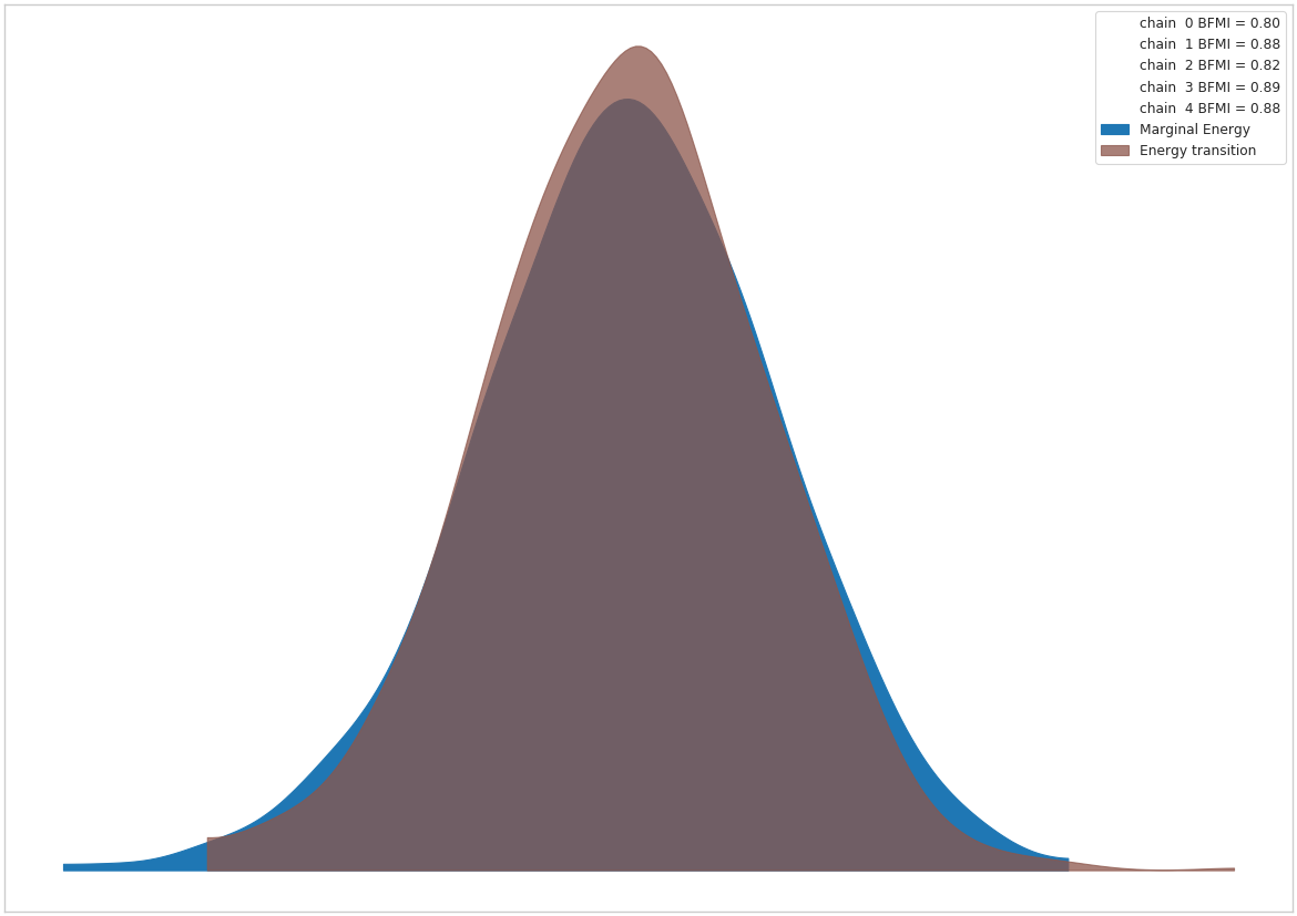
Fig. 5 Post-transform MCMC energy

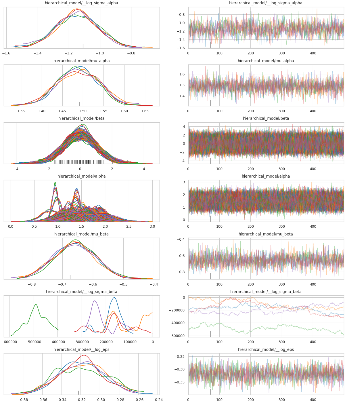
Fig. 6 Post-transform MCMC trace

Discussion

The goals in the two separate run calls we used in kanren-shift-squaredo-func could have been combined into a single run. This could’ve been accomplished using some “meta” steps (e.g. construct and evaluate a goal on-the-fly within a miniKanren) or special goals for reading from a miniKanren-generated dicts or association lists. Goals of this nature are not uncommon (e.g. type inference and inhabitation exmaples), and serve to demonstrate the great breadth of activity possible within relational context of miniKanren.

However, the point we want to make doesn’t require much sophistication. Instead, we wanted to demonstrate how a non-trivial “pattern” can be specified and matched using symbolic-pymc, and how easily those results could be used to transform a graph.

More specifically, our goal shift_squared_subso in kanren-shift-squaredo-func demonstrates the way in which we were able to specify desired structure(s) within a graph. We defined one pattern, Y_sqrdiffo, to match anywhere in the graph then another pattern, X_sqrdiffo, that relied on matched terms from Y_sqrdiffo and could also be matched/found anywhere else in the same graph.

Furthermore, our substitutions needed information from both “matched” subgraphs. Specifically, substitution pairs similar to (x, z + x). Within this framework, we could just as easily have included y–or any terms from either successfully matched subgraph–in the substitution expressions.

In sample-space, the search patterns and substitutions are much easier to specify exactly because they’re single-subgraph patterns that themselves are the subgraphs to be replaced (i.e. if we find a non-standard normal, replace it with a shifted/scaled standard normal). In log-space, we chose to find distinct subgraph “chains”, i.e. all (y - x)**2and (x - z)**2 pairs (i.e. “connected” by an “unknown” term x), since these are produced by the log-likelihood form of hierarchical normal distributions.

As a result, we had a non-trivial structure/”pattern” to express–and execute. Using conventional graph search-and-replace functionality would’ve required much more orchestration and resulted considerably less flexible code with little-to-no reusability. In our case, the goals onceo and walkoare universal and the forms in shift_squared_subso can be easily changed to account for more sophisticated (or entirely distinct) patterns and substitutions.

Most related graph manipulation offerings make it easy to find a single subgraph that matches a pattern, but not potentially “co-dependent” and/or distinct subgraphs. In the end, the developer will often have to manually implement a “global” state and orchestrate multiple single-subgraph searches and their results.

For single search-and-replace objectives, this amount of manual developer intervention/orchestration might be excusable; however, for objectives requiring the evaluation of multiple graph transformation, this approach is mostly unmaintainable and extremely difficult to compartmentalize.

This demonstration barely even scratches the surface of what’s possible using miniKanren and relational programming for graph manipulation and symbolic statistical model optimization. As the symbolic-pymcproject advances, we’ll cover examples in which miniKanren’s more distinct offerings are demonstrated.