Usage with Stan models

This document shows how to use nutpie with Stan models. We will use the nutpie package to define a simple model and sample from it using Stan.

Installation

For Stan, it is more common to use pip or uv to install the necessary packages. However, conda is also an option if you prefer.

To install using pip:

pip install "nutpie[stan]"

To install using uv:

uv add "nutpie[stan]"

To install using conda:

conda install -c conda-forge nutpie

Compiler Toolchain

Stan requires a compiler toolchain to be installed on your system. This is necessary for compiling the Stan models. You can find detailed instructions for setting up the compiler toolchain in the CmdStan Guide.

Additionally, since Stan uses Intel’s Threading Building Blocks (TBB) for parallelism, you might need to set the TBB_CXX_TYPE environment variable to specify the compiler type. Depending on your system, you can set it to either clang or gcc. For example:

import os
os.environ["TBB_CXX_TYPE"] = "clang"  # or 'gcc'

Make sure to set this environment variable before compiling your Stan models to ensure proper configuration.

Defining and Sampling a Simple Model

We will define a simple Bayesian model using Stan and sample from it using nutpie.

Model Definition

In your Python script or Jupyter notebook, add the following code:

import nutpie

model_code = """
data {
    int<lower=0> N;
    vector[N] y;
}
parameters {
    real mu;
}
model {
    mu ~ normal(0, 1);
    y ~ normal(mu, 1);
}
"""

compiled_model = nutpie.compile_stan_model(code=model_code)

BridgeStan not found at location specified by $BRIDGESTAN environment variable, downloading version 2.9.0 to /home/runner/.bridgestan/bridgestan-2.9.0
Done!

Sampling

We can now compile the model and sample from it:

compiled_model_with_data = compiled_model.with_data(N=3, y=[1, 2, 3])
trace = nutpie.sample(compiled_model_with_data)

Sampler Progress

Total Chains: 6

Active Chains: 0

Finished Chains: 6

Sampling for now

Estimated Time to Completion: now

Draws	Step Size	Gradients/Draw	Log Fisher
1400	1.47	1	-68.87
1400	1.16	1	-68.20
1400	1.24	1	-68.06
1400	1.25	3	-70.25
1400	1.36	3	-68.87
1400	1.21	1	-68.87

Using Dimensions

We’ll use the radon model from this case-study from the stan documentation, to show how we can use coordinates and dimension names to simplify working with trace objects.

We follow the same data preparation as in the case-study:

import pandas as pd
import numpy as np
import arviz as az
import seaborn as sns

home_data = pd.read_csv(
    "https://github.com/pymc-devs/pymc-examples/raw/refs/heads/main/examples/data/srrs2.dat",
    index_col="idnum",
)
county_data = pd.read_csv(
    "https://github.com/pymc-devs/pymc-examples/raw/refs/heads/main/examples/data/cty.dat",
)

radon_data = (
    home_data
    .rename(columns=dict(cntyfips="ctfips"))
    .merge(
        (
            county_data
            .drop_duplicates(['stfips', 'ctfips', 'st', 'cty', 'Uppm'])
            .set_index(["ctfips", "stfips"])
        ),
        right_index=True,
        left_on=["ctfips", "stfips"],
    )
    .assign(log_radon=lambda x: np.log(np.clip(x.activity, 0.1, np.inf)))
    .assign(log_uranium=lambda x: np.log(np.clip(x["Uppm"], 0.1, np.inf)))
    .query("state == 'MN'")
)

And also use the partially pooled model from the case-study:

model_code = """
data {
  int<lower=1> N;  // observations
  int<lower=1> J;  // counties
  array[N] int<lower=1, upper=J> county;
  vector[N] x;
  vector[N] y;
}
parameters {
  real mu_alpha;
  real<lower=0> sigma_alpha;
  vector<offset=mu_alpha, multiplier=sigma_alpha>[J] alpha;  // non-centered parameterization
  real beta;
  real<lower=0> sigma;
}
model {
  y ~ normal(alpha[county] + beta * x, sigma);
  alpha ~ normal(mu_alpha, sigma_alpha); // partial-pooling
  beta ~ normal(0, 10);
  sigma ~ normal(0, 10);
  mu_alpha ~ normal(0, 10);
  sigma_alpha ~ normal(0, 10);
}
generated quantities {
  array[N] real y_rep = normal_rng(alpha[county] + beta * x, sigma);
}
"""

We collect the dataset in the format that the stan model requires, and specify the dimensions of each of the non-scalar variables in the model:

county_idx, counties = pd.factorize(radon_data["county"], use_na_sentinel=False)
observations = radon_data.index

coords = {
    "county": counties,
    "observation": observations,
}

dims = {
    "alpha": ["county"],
    "y_rep": ["observation"],
}

data = {
    "N": len(observations),
    "J": len(counties),
    # Stan uses 1-based indexing!
    "county": county_idx + 1,
    "x": radon_data.log_uranium.values,
    "y": radon_data.log_radon.values,
}

Then, we compile the model and provide the dimensions, coordinates and the dataset we just defined:

compiled_model = (
    nutpie.compile_stan_model(code=model_code)
    .with_data(**data)
    .with_dims(**dims)
    .with_coords(**coords)
)

%%time
trace = nutpie.sample(compiled_model, seed=0)

Sampler Progress

Total Chains: 6

Active Chains: 0

Finished Chains: 6

Sampling for now

Estimated Time to Completion: now

Draws	Step Size	Gradients/Draw	Log Fisher
1400	0.50	7	1.46
1400	0.52	7	1.92
1400	0.46	7	1.99
1400	0.46	7	0.62
1400	0.42	15	2.47
1400	0.48	15	2.24

CPU times: user 3.7 s, sys: 65.7 ms, total: 3.77 s
Wall time: 1.31 s

As some basic convergance checking we verify that all Rhat values are smaller than 1.02, all parameters have at least 500 effective draws and that we have no divergences:

assert trace.sample_stats.diverging.sum() == 0
assert az.ess(trace).min().min() > 500
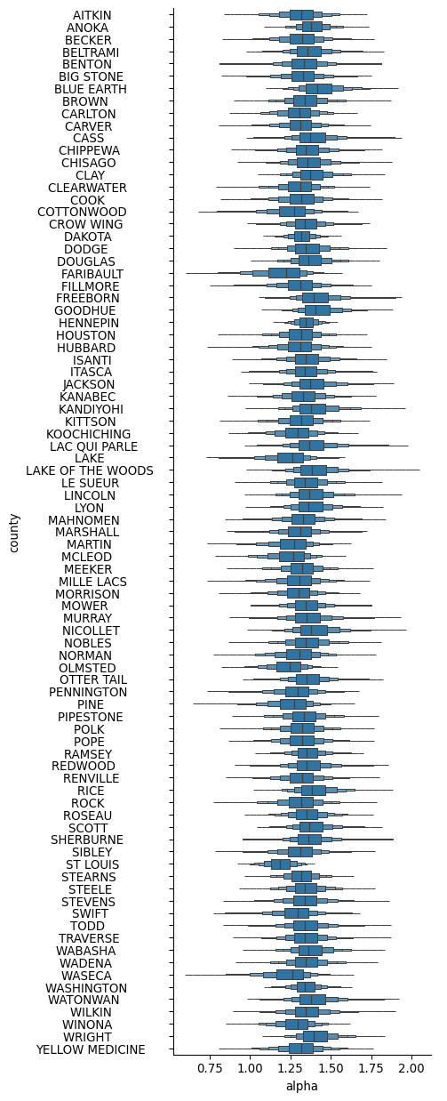
assert az.rhat(trace).max().max() > 1.02

Thanks to the coordinates and dimensions we specified, the resulting trace will now contain labeled data, so that plots based on it have properly set-up labels:

import arviz as az
import seaborn as sns
import xarray as xr

sns.catplot(
    data=trace.posterior.alpha.to_dataframe().reset_index(),
    y="county",
    x="alpha",
    kind="boxen",
    height=13,
    aspect=1/2.5,
    showfliers=False,
)

Initial points

By default, every chain starts at a point drawn from a standard normal distribution on the unconstrained space. You can replace this with your own function using with_init_point_fn. The function is called as init_point_fn(model, rng, chain_id), where model is the compiled model that is sampled, rng is a numpy.random.Generator and chain_id is the index of the chain.

The simplest option is to return a dictionary with values for some or all parameters of the model, on the constrained space. Parameters that are not in the dictionary are drawn uniformly from \([-2, 2]\) on the unconstrained space, just as Stan does it:

model_code = """
data {
    int<lower=0> N;
    vector[N] y;
}
parameters {
    real mu;
    real<lower=0> sigma;
}
model {
    mu ~ normal(0, 10);
    sigma ~ normal(0, 1);
    y ~ normal(mu, sigma);
}
"""

compiled_model = (
    nutpie.compile_stan_model(code=model_code)
    .with_data(N=3, y=[1, 2, 3])
)

def init_point(model, rng, chain_id):
    # Start mu at the mean of the data, and let nutpie choose sigma
    return {"mu": 2.0 + rng.normal(scale=0.1)}

trace = nutpie.sample(compiled_model.with_init_point_fn(init_point))

Sampler Progress

Total Chains: 6

Active Chains: 0

Finished Chains: 6

Sampling for now

Estimated Time to Completion: now

Draws	Divergences	Step Size	Gradients/Draw	Log Fisher
1400	1	0.79	7	-1.54
1400	0	0.96	3	-0.24
1400	1	1.00	7	-0.18
1400	0	0.97	3	-0.12
1400	0	0.83	3	-2.72
1400	1	0.84	3	-1.16

Alternatively, the function can return a flat array on the unconstrained space, with shape (model.n_dim,). unconstrain computes such a point from constrained values, and constrain maps it back to the flat vector of constrained values, in the order used by Stan:

point = compiled_model.unconstrain(mu=2.0, sigma=0.5)
point

array([ 2.        , -0.69314718])

compiled_model.constrain(point)

array([2. , 0.5])

If the log density at a returned point is not finite, the function is called again with a new rng, up to 500 times per chain. Values that violate the constraints of a parameter, for instance a negative sigma, are treated the same way. For those, Stan currently prints a message for each rejected attempt.